Markov chains

This page shows how the results of Lesson 4 might be obtained using Markov chains. Note that this is not how QPLEX does it.

To review, here are the engine attributes from Lesson 4:

engine.number_of_arrivals_pmf = {2: 0.3, 3: 0.7}
engine.service_duration_pmf = {1: 0.6, 2: 0.3, 3: 0.1}
engine.number_of_servers = 2

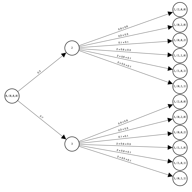
This system can be represented as a Markov chain, so long as the state is allowed to take an unusually elaborate form. Here is an example of a state:

(5, (1, 0, 1))

The first entry (5) specifies the number of entities in the system. The second entry is a histogram, representing the number of entities in service that have remaining service duration of 1, 2, or 3, respectively. For this particular histogram, one of the servers has a remaining service duration of one, while the other has a remaining service duration of three.

The initial system state is represented as (0, (0, 0, 0)) since the system is initially empty. The figure below shows the reachable states from this initial state after a single transition:

The pmf of the state of the Markov chain at time 1 is more naturally summarized in a table:

z	Prob(z)	(2,0,0)	(0,2,0)	(0,0,2)	(1,1,0)	(1,0,1)	(0,1,1)
2	0.30000	0.36000	0.09000	0.01000	0.36000	0.12000	0.06000
3	0.70000	0.36000	0.09000	0.01000	0.36000	0.12000	0.06000

In this table, z represents the number of entities in the system. Each entry in row z and column h represents the conditional probability of state (z, h) given z.

As noted in Lesson 4, the number in the system at time 1 equals the number of arrivals during the first period, so the marginal distribution of z (second column) equals the number of arrivals pmf.

Here is the pmf of the state of the Markov chain at time 2:

z	Prob(z)	(2,0,0)	(0,2,0)	(0,0,2)	(1,1,0)	(1,0,1)	(0,1,1)
2	0.03240	0.36000	0.09000	0.01000	0.36000	0.12000	0.06000
3	0.19440	0.38000	0.08667	0.00778	0.36333	0.11000	0.05222
4	0.39240	0.41367	0.08128	0.00450	0.36826	0.09248	0.03982
5	0.30240	0.47500	0.07222	0.00000	0.37500	0.05833	0.01944
6	0.07840	0.56250	0.06250	0.00000	0.37500	0.00000	0.00000

The pmf of the number of entities in the system at time 2 exactly matches the QPLEX output. It might not be obvious, but it is now confirmed by computing two different ways.

Here is the pmf of the state of the Markov chain at time 3:

z	Prob(z)	(2,0,0)	(0,2,0)	(0,0,2)	(1,1,0)	(1,0,1)	(0,1,1)
2	0.00350	0.36000	0.09000	0.01000	0.36000	0.12000	0.06000
3	0.03499	0.37200	0.08800	0.00867	0.36200	0.11400	0.05533
4	0.14045	0.38898	0.08455	0.00715	0.36324	0.10669	0.04940
5	0.28755	0.41450	0.07839	0.00545	0.36229	0.09767	0.04169
6	0.31439	0.45621	0.06691	0.00362	0.35536	0.08642	0.03148
7	0.17423	0.53327	0.04429	0.00177	0.33107	0.07188	0.01772
8	0.04145	0.70213	0.00000	0.00000	0.24823	0.04965	0.00000
9	0.00343	1.000000	0.00000	0.00000	0.00000	0.00000	0.00000

And here is the comparison with QPLEX:

z	Markov Prob(z)	QPLEX Prob(z)
2	0.00350	0.00350
3	0.03499	0.03501
4	0.14045	0.14059
5	0.28755	0.28784
6	0.31439	0.31405
7	0.17423	0.17341
8	0.04145	0.04217
9	0.00343	0.00343

This time, the results from the Markov analysis do not exactly match the results from QPLEX. That's because QPLEX is an approximate methodology.

But they are very close.

Unfortunately, the Markov chain approach is unworkable for all but trivial systems, because the number of states is \(O(L^n)\), where n is the number of servers, and L is the number of possible service durations. This is known as the curse of dimensionality.

QPLEX, of course, does not use the Markov chain method, so it is not affected by the number of states of the Markov model. An overview of how it accomplishes this may be found on the next page.